Inverse Mie Theory Functions¶

Contour Intersection Inversion Functions¶

For more details on the contour intersection inversion method, please see Sumlin BJ, Heinson WR, Chakrabarty RK. Retrieving the Aerosol Complex Refractive Index using PyMieScatt: A Mie Computational Package with Visualization Capabilities. J. Quant. Spectros. Rad. Trans. 2017. DOI: 10.1016/j.jqsrt.2017.10.012 There’s also a good example here.

ContourIntersection(Qsca, Qabs, wavelength, diameter[, n=None, k=None, nMin=1, nMax=3, kMin=0.00001, kMax=1, Qback=None, gridPoints=100, interpolationFactor=2, maxError=0.005, fig=None, ax=None, axisOption=0])¶

Computes complex m = n+ik from a particle diameter (in nm), incident wavelength (in nm), and scattering and absorption efficiencies. Optionally, backscatter efficiency may be specified to constrain the problem to produce a unique solution.

Parameters

Qsca : float or list-like

The scattering efficiency, or optionally, a list, tuple, or numpy.ndarray of scattering efficiency and its associated error.

Qabs : float or list-like

The absorption efficiency, or optionally, a list, tuple, or numpy.ndarray of absorption efficiency and its associated error..

wavelength : float

The wavelength of incident light, in nm.

diameter : float

The diameter of the particle, in nm.

n : float or list-like, optional

An assumed real refractive index. Can be used in case scattering data is not available. If specified as a list, it must have only two elements. The first is the assumed n and the second is an uncertainty, such as a standard deviation.

k : float or list-like, optional

An assumed imaginary refractive index. Useful if only considering nonabsorbing aerosols, so you can set k=0. If specified as a list, it must have only two elements. The first is the assumed k and the second is an uncertainty, such as a standard deviation. **Note: when specifying this in the function call, input it as a real number. Omit the imaginary unit.

nMin : float, optional

The minimum value of n to search.

nMax : float, optional

The maximum value of n to search.

kMin : float, optional

The minimum value of k to search.

kMax : float, optional

The maximum value of k to search.

Qback : float or list-like, optional

The backscatter efficiency, or optionally, a list, tuple, or numpy.ndarray of backscatter efficiency and its associated error.

gridPoints : int, optional

The number of gridpoints for the search mesh. Defaults to 200. Increase for better resolution but longer run times.

interpolationFactor : int, optional

The interpolation to apply to the search fields, artificially increasing their resolutions. This is applied after calculations, so some features may be lost if interpolationFactor is too high and gridPoints is too low.

maxError : float, optional

The allowed error in forward calculations of the retrived m.

fig : matplotlib.figure object, optional (but recommended)

The figure object to send to the geometric inversion routine. If unspecified, one will be created.

ax : matplotlib.axes object, optional (but recommended)

The axes object to send to the geometric inversion routine. If unspecified, one will be created.

axisOption : int, optional

Dictates the axis scales. Kind of useless since version 1.3.0. It’s still around until I get rid of it. Acceptable parameters are:

‘0’ for automatic detection of best axis scaling
‘1’ for linear axes
‘2’ for linear x and logarithmic y
‘3’ for logarithmic x and linear y
‘4’ for log-log

Returns

solutionSet : list

A list of all valid solutions

ForwardCalculations : list

A list of scattering and absorption efficencies produced by forward Mie calculations using the derived refractive indices

solutionErrors : list

The relative errors of the efficencies in ForwardCalculations.

fig : matplotlib.figure object

The figure object now associated with the inversion calculations.

ax : matplotlib.axes object

The axes object now associated with the inversion calculations.

graphElements : dict

A dict of all artists necessary to fully manipulate the appearance of the output. The keys will depend on the options passed to the inversion function itself (i.e., errors specified, backscatter specified). Maximally, it will contain:

‘Qsca’, ‘Qabs’, ‘Qback’ - the major contours;
‘QscaErrFill’, ‘QscaErrOutline1’, ‘QscaErrOutline2’ - the error bound contours;
‘QabsErrFill’, ‘QabsErrOutline1’, ‘QabsErrOutline2’ - the error bound fills;
‘SolMark’, ‘SolFill’ - the circle thingies at each solution;
‘CrosshairsH’, ‘CrosshairsV’ - solution crosshairs;
‘LeftSpine’, ‘RightSpine’, ‘BottomSpine’, ‘TopSpine’ - graph spines;
‘XAxis’, ‘YAxis’ - the individual matplotlib axis objects.

ContourIntersection_SD(Bsca, Babs, wavelength, dp, ndp[, n=None, k=None, nMin=1, nMax=3, kMin=0.00001, kMax=1, SMPS=True, Bback=None, gridPoints=100, interpolationFactor=2, maxError=0.005, fig=None, ax=None, axisOption=0])¶

Computes effective complex m = n+ik from a measured or constructed size distribution (in cm^-3), incident wavelength (in nm), and scattering and absorption coefficients (in Mm^-1). Optionally, backscatter coefficient may be specified to constrain the problem to produce a unique solution.

Parameters

Bsca : float or list-like

The scattering coefficient, or optionally, a list, tuple, or numpy.ndarray of scattering coefficient and its associated error.

Babs : float or list-like

The absorption coefficient, or optionally, a list, tuple, or numpy.ndarray of absorption coefficient and its associated error..

wavelength : float

The wavelength of incident light, in nm.

dp : list-like

The diameter bins of the size distribution, in nm.

ndp : list-like

The number of particles per diameter bin corresponding to dp, in cm^-3. Must be same length as dp.

n : float or list-like, optional

An assumed real refractive index. Can be used in case scattering data is not available. If specified as a list, it must have only two elements. The first is the assumed n and the second is an uncertainty, such as a standard deviation.

k : float or list-like, optional

An assumed imaginary refractive index. Useful if only considering nonabsorbing aerosols, so you can set k=0. If specified as a list, it must have only two elements. The first is the assumed k and the second is an uncertainty, such as a standard deviation. **Note: when specifying this in the function call, input it as a real number. Omit the imaginary unit.

nMin : float, optional

The minimum value of n to search.

nMax : float, optional

The maximum value of n to search.

kMin : float, optional

The minimum value of k to search.

kMax : float, optional

The maximum value of k to search.

SMPS : bool, optional

The switch determining the source of the size distribution data. Omit or set to True for laboratory measurements, set to False for analytical distributions.

Bback : float or list-like, optional

The backscatter coefficient, or optionally, a list, tuple, or numpy.ndarray of backscatter coefficient and its associated error.

gridPoints : int, optional

The number of gridpoints for the search mesh. Defaults to 200. Increase for better resolution but longer run times.

interpolationFactor : int, optional

The interpolation to apply to the search fields, artificially increasing their resolutions. This is applied after calculations, so some features may be lost if interpolationFactor is too high and gridPoints is too low.

maxError : float, optional

The allowed error in forward calculations of the retrived m.

fig : matplotlib.figure object, optional (but recommended)

The figure object to send to the geometric inversion routine. If unspecified, one will be created.

ax : matplotlib.axes object, optional (but recommended)

The axes object to send to the geometric inversion routine. If unspecified, one will be created.

axisOption : int, optional

Dictates the axis scales. Kind of useless since version 1.3.0. It’s still around until I get rid of it. Acceptable parameters are:

‘0’ for automatic detection of best axis scaling
‘1’ for linear axes
‘2’ for linear x and logarithmic y
‘3’ for logarithmic x and linear y
‘4’ for log-log

Returns

solutionSet : list

A list of all valid solutions

ForwardCalculations : list

A list of scattering and absorption coefficients produced by forward Mie calculations using the derived effective refractive indices

solutionErrors : list

The relative errors of the coefficients in ForwardCalculations.

fig : matplotlib.figure object

The figure object now associated with the inversion calculations.

ax : matplotlib.axes object

The axes object now associated with the inversion calculations.

graphElements : dict

A dict of all artists necessary to fully manipulate the appearance of the output. The keys will depend on the options passed to the inversion function itself (i.e., errors specified, backscatter specified). Maximally, it will contain:

‘Bsca’, ‘Babs’, ‘Bback’ - the major contours;
‘BscaErrFill’, ‘BscaErrOutline1’, ‘BscaErrOutline2’ - the error bound contours;
‘BabsErrFill’, ‘BabsErrOutline1’, ‘BabsErrOutline2’ - the error bound fills;
‘SolMark’, ‘SolFill’ - the circle thingies at each solution;
‘CrosshairsH’, ‘CrosshairsV’ - solution crosshairs;
‘LeftSpine’, ‘RightSpine’, ‘BottomSpine’, ‘TopSpine’ - graph spines;
‘XAxis’, ‘YAxis’ - the individual matplotlib axis objects.

Survey-iteration Inversion Functions¶

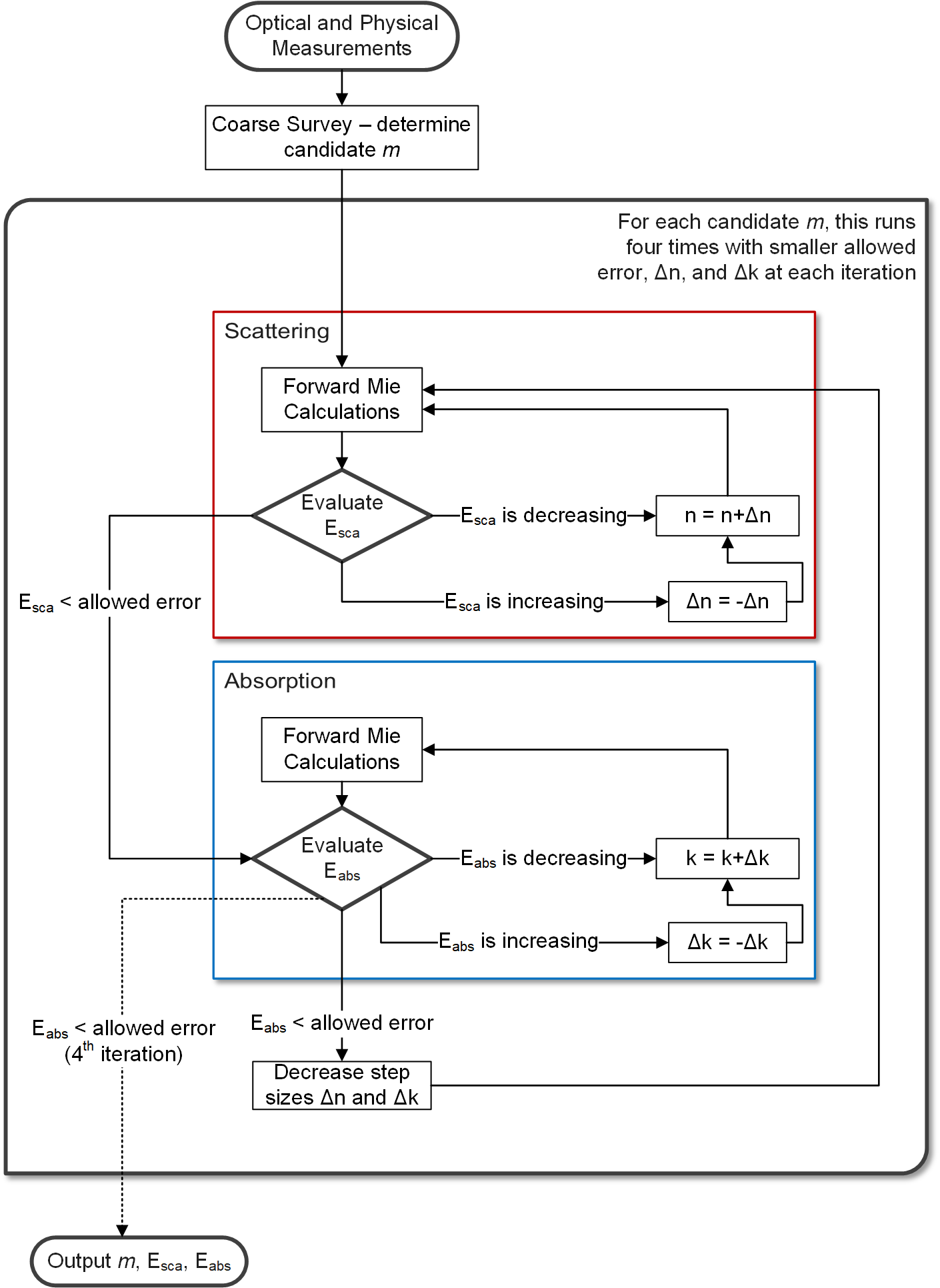
The survey-iteration inversion algorithm is discussed in detail in the Supplementary Material of the JQSRT paper. It is a strictly numerical two phase algorithm. First, a low-resolution survey of n-k space is conducted and values of efficiencies or coefficients close to the inputs are located. From this survey, candidate m values are determined. The iteration phase is best described by this flowchart:

SurveyIteration(Qsca, Qabs, wavelength, diameter[, tolerance=0.0005])¶

Computes complex m=n+ik for given scattering and absorption efficencies, incident wavelength, and particle diameter.

Parameters

Qsca : float: Measured scattering efficiency.
Qabs : float: Measured absorption efficiency.
wavelength : float: The incident wavelength of light, in nm.
diameter : float: The particle diameter in nm.
tolerance : float, optional: The maximum error allowed in forward Mie calculations of retrieved indices.

Returns

resultM : list-like: The retrieved refractive indices. Be sure and scrutinize this list for repeat entries.
resultScaErr : list-like: The relative error in scattering efficiency for each retrieved m.
resultAbsErr : list-like: The relative error in absorption efficiency for each retrieved m.

SurveyIteration_SD(Bsca, Babs, wavelength, dp, ndp[, tolerance=0.0005, SMPS=True])¶

Computes complex m=n+ik for given scattering and absorption coefficients, incident wavelength, and particle diameter.

Parameters

Qsca : float: Measured scattering coefficient.
Qabs : float: Measured absorption coefficient.
wavelength : float: The incident wavelength of light, in nm.
dp : list-like: The particle diameter bins in nm.
ndp : list-like: The particle concentrations (in cm^-3) corresponding to each of the bins in dp.
tolerance : float, optional: The maximum error allowed in forward Mie calculations of retrieved indices.
SMPS : bool, optional: The switch determining the source of the size distribution data. Omit or set to True for laboratory measurements, set to False for analytical distributions.

Returns

resultM : list-like: The retrieved refractive indices. Be sure and scrutinize this list for repeat entries.
resultScaErr : list-like: The relative error in scattering coefficient for each retrieved m.
resultAbsErr : list-like: The relative error in absorption coefficient for each retrieved m.