Functions for Forward Mie Calculations of Homogeneous Spheres¶

Functions for single particles¶

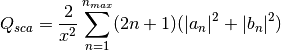
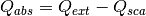
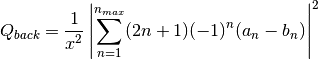
MieQ(m, wavelength, diameter[, nMedium=1.0, asDict=False, asCrossSection=False])¶

Computes Mie efficencies Q and asymmetry parameter g of a single, homogeneous particle. Uses Mie_ab() to calculate $a_n$ and $b_n$ , and then calculates Q via:

$Q_{ext}=\frac{2}{x^2}\sum_{n=1}^{n_{max}}(2n+1)\:\text{Re}\left\{a_n+b_n\right\}$

$Q_{sca}=\frac{2}{x^2}\sum_{n=1}^{n_{max}}(2n+1)(|a_n|^2+|b_n|^2)$

$Q_{abs}=Q_{ext}-Q_{sca}$

$Q_{back}=\frac{1}{x^2} \left| \sum_{n=1}^{n_{max}}(2n+1)(-1)^n(a_n-b_n) \right| ^2$

$Q_{ratio}=\frac{Q_{back}}{Q_{sca}}$

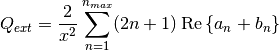
$g=\frac{4}{Q_{sca}x^2}\left[\sum\limits_{n=1}^{n_{max}}\frac{n(n+2)}{n+1}\text{Re}\left\{a_n a_{n+1}^*+b_n b_{n+1}^*\right\}+\sum\limits_{n=1}^{n_{max}}\frac{2n+1}{n(n+1)}\text{Re}\left\{a_n b_n^*\right\}\right]$

$Q_{pr}=Q_{ext}-gQ_{sca}$

where asterisks denote the complex conjugates.

Parameters

m : complex: The complex refractive index, with the convention m = n+ik.
wavelength : float: The wavelength of incident light, in nanometers.
diameter : float: The diameter of the particle, in nanometers.
nMedium : float, optional: The refractive index of the surrounding medium. This must be positive, nonzero, and real. Any imaginary part will be discarded.
asDict : bool, optional: If specified and set to True, returns the results as a dict.
asCrossSection : bool, optional: If specified and set to True, returns the results as optical cross-sections with units of nm².

Returns

qext, qsca, qabs, g, qpr, qback, qratio : float: The Mie efficencies described above.
cext, csca, cabs, g, cpr, cback, cratio : float: If asCrossSection==True, MieQ() returns optical cross-sections with units of nm².
q : dict: If asDict==True, MieQ() returns a dict of the above efficiencies with appropriate keys.
c : dict: If asDict==True and asCrossSection==True, returns a dict of the above cross-sections with appropriate keys.

For example, compute the Mie efficencies of a particle 300 nm in diameter with m = 1.77+0.63i, illuminated by λ = 375 nm:

>>> import PyMieScatt as ps
>>> ps.MieQ(1.77+0.63j,375,300,asDict=True)
{'Qext': 2.8584971991564112,
 'Qsca': 1.3149276685170939,
 'Qabs': 1.5435695306393173,
 'g': 0.7251162362148782,
 'Qpr': 1.9050217972664911,
 'Qback': 0.20145510481352547,
 'Qratio': 0.15320622543498222}

Mie_ab(m, x)¶

Computes external field coefficients a_n and b_n based on inputs of m and $x=\pi\,d_p/\lambda$ . Must be explicitly imported via

>>> from PyMieScatt.Mie import Mie_ab

Parameters

m : complex

The complex refractive index with the convention m = n+ik.

x : float

The size parameter $x=\pi\,d_p/\lambda$ .

Returns

an, bn : numpy.ndarray

Arrays of size n_max = 2+x+4x^1/3

Mie_cd(m, x)¶

Computes internal field coefficients c_n and d_n based on inputs of m and $x=\pi\,d_p/\lambda$ . Must be explicitly imported via
>>> from PyMieScatt.Mie import Mie_cd

Parameters

m : complex

The complex refractive index with the convention m = n+ik.

x : float

The size parameter $x=\pi\,d_p/\lambda$ .

Returns

cn, dn : numpy.ndarray

Arrays of size n_max = 2+x+4x^1/3

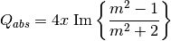
RayleighMieQ(m, wavelength, diameter[, nMedium=1.0, asDict=False, asCrossSection=False])¶

Computes Mie efficencies of a spherical particle in the Rayleigh regime ( $x=\pi\,d_p/\lambda \ll 1$ ) given refractive index m, wavelength, and diameter. Optionally returns the parameters as a dict when asDict is specified and set to True. Uses Rayleigh-regime approximations:

$Q_{sca}=\frac{8x^4}{3}\left|{\frac{m^2-1}{m^2+2}}\right|^2$

$Q_{abs}=4x\:\text{Im}\left\{\frac{m^2-1}{m^2+2}\right\}$

$Q_{ext}=Q_{sca}+Q_{abs}$

$Q_{back}=\frac{3Q_{sca}}{2}$

$Q_{ratio}=1.5$

$Q_{pr}=Q_{ext}$

Parameters

m : complex: The complex refractive index, with the convention m = n+ik.
wavelength : float: The wavelength of incident light, in nanometers.
diameter : float: The diameter of the particle, in nanometers.
nMedium : float, optional: The refractive index of the surrounding medium. This must be positive, nonzero, and real. Any imaginary part will be discarded.
asDict : bool, optional: If specified and set to True, returns the results as a dict.
asCrossSection : bool, optional: If specified and set to True, returns the results as optical cross-sections with units of nm².

Returns

qext, qsca, qabs, g, qpr, qback, qratio : float: The Mie efficencies described above.
cext, csca, cabs, g, cpr, cback, cratio : float: If asCrossSection==True, RayleighMieQ() returns optical cross-sections.
q : dict: If asDict==True, RayleighMieQ() returns a dict of the above efficiencies with appropriate keys.
c : dict: If asDict==True and asCrossSection==True, returns a dict of the above cross-sections with appropriate keys.

For example, compute the Mie efficencies of a particle 50 nm in diameter with m = 1.33+0.01i, illuminated by λ = 870 nm:

>>> import PyMieScatt as ps
>>> ps.MieQ(1.33+0.01j,870,50,asDict=True)
{'Qabs': 0.004057286640269908,
 'Qback': 0.00017708468873118297,
 'Qext': 0.0041753430994240295,
 'Qpr': 0.0041753430994240295,
 'Qratio': 1.5,
 'Qsca': 0.00011805645915412197,
 'g': 0}

AutoMieQ(m, wavelength, diameter[, nMedium=1.0, crossover=0.01, asDict=False, asCrossSection=False])¶

Returns Mie efficencies of a spherical particle according to either MieQ() or RayleighMieQ() depending on the magnitude of the size parameter. Good for studying parameter ranges or size distributions. Thanks to John Kendrick for discussions about where to best place the crossover point.

Parameters

m : complex: The complex refractive index, with the convention m = n+ik.
wavelength : float: The wavelength of incident light, in nanometers.
diameter : float: The diameter of the particle, in nanometers.
nMedium : float, optional: The refractive index of the surrounding medium. This must be positive, nonzero, and real. Any imaginary part will be discarded.
crossover : float, optional: The size parameter that dictates where calculations switch from Rayleigh approximation to actual Mie.
asDict : bool, optional: If specified and set to True, returns the results as a dict.
asCrossSection : bool, optional: If specified and set to True, returns the results as optical cross-sections with units of nm².

Returns

qext, qsca, qabs, g, qpr, qback, qratio : float: The Mie efficencies described above.
cext, csca, cabs, g, cpr, cback, cratio : float: If asCrossSection==True, AutoMieQ() returns optical cross-sections.
q : dict: If asDict==True, AutoMieQ() returns a dict of the above efficiencies with appropriate keys.
c : dict: If asDict==True and asCrossSection==True, returns a dict of the above cross-sections with appropriate keys.

LowFrequencyMieQ(m, wavelength, diameter[, nMedium=1.0, asDict=False, asCrossSection=False])¶

Returns Mie efficencies of a spherical particle in the low-frequency regime ( $x=\pi\,d_p/\lambda \ll 1$ ) given refractive index m, wavelength, and diameter. Optionally returns the parameters as a dict when asDict is specified and set to True. Uses LowFrequencyMie_ab() to calculate a_n and b_n, and follows the same math as MieQ().

Parameters

m : complex: The complex refractive index, with the convention m = n+ik.
wavelength : float: The wavelength of incident light, in nanometers.
diameter : float: The diameter of the particle, in nanometers.
nMedium : float, optional: The refractive index of the surrounding medium. This must be positive, nonzero, and real. Any imaginary part will be discarded.
asDict : bool, optional: If specified and set to True, returns the results as a dict.
asCrossSection : bool, optional: If specified and set to True, returns the results as optical cross-sections with units of nm².

Returns

qext, qsca, qabs, g, qpr, qback, qratio : float: The Mie efficencies described above.
cext, csca, cabs, g, cpr, cback, cratio : float: If asCrossSection==True, LowFrequencyMieQ() returns optical cross-sections.
q : dict: If asDict==True, LowFrequencyMieQ() returns a dict of the above efficiencies with appropriate keys.
c : dict: If asDict==True and asCrossSection==True, returns a dict of the above cross-sections with appropriate keys.

For example, compute the Mie efficencies of a particle 100 nm in diameter with m = 1.33+0.01i, illuminated by λ = 1600 nm:

>>> import PyMieScatt as ps
>>> ps.LowFrequencyMieQ(1.33+0.01j,1600,100,asDict=True)
{'Qabs': 0.0044765816617916582,
 'Qback': 0.00024275862007727458,
 'Qext': 0.0046412326004135135,
 'Qpr': 0.0046400675577583459,
 'Qratio': 1.4743834569616665,
 'Qsca': 0.00016465093862185558,
 'g': 0.0070758336692078412}

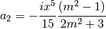
LowFrequencyMie_ab(m, x)¶

Returns external field coefficients a_n and b_n based on inputs of m and $x=\pi\,d_p/\lambda$ by limiting the expansion of a_n and b_n to second order:

$a_1=\frac{m^2-1}{m^2+2} \left[ -\frac{i2x^3}{3}-\frac{2ix^5}{5}\left( \frac{m^2-2}{m^2+2}\right) +\frac{4x^6}{9}\left( \frac{m^2-1}{m^2+2} \right) \right]$

$a_2=-\frac{ix^5}{15}\frac{(m^2-1)}{2m^2+3}$

$b_1=-\frac{ix^5}{45}(m^2-1)$

$b_2=0$

Parameters

m : complex

The complex refractive index with the convention m = n+ik.

x : float

The size parameter $x=\pi\,d_p/\lambda$ .

Returns

an, bn : numpy.ndarray

Arrays of size 2.

Functions for single particles across various ranges¶

MieQ_withDiameterRange(m, wavelength[, nMedium=1.0, diameterRange=(10, 1000), nd=1000, logD=False])¶

Computes the Mie efficencies of particles across a diameter range using AutoMieQ().

Parameters

m : complex: The complex refractive index with the convention m = n+ik.
wavelength : float: The wavelength of incident light, in nanomaters
nMedium : float, optional: The refractive index of the surrounding medium. This must be positive, nonzero, and real. Any imaginary part will be discarded.
diameterRange : tuple or list, optional: The diameter range, in nanometers. Convention is (smallest, largest). Defaults to (10, 1000).
nd : int, optional: The number of diameter bins in the range. Defaults to 1000.
logD : bool, optional: If True, will use logarithmically-spaced diameter bins. Defaults to False.

Returns

diameters : numpy.ndarray: An array of the diameter bins that calculations were performed on. Size is equal to nd.
qext, qsca, qabs, g, qpr, qback, qratio : numpy.ndarray: The Mie efficencies at each diameter in diameters.

MieQ_withWavelengthRange(m, diameter[, nMedium=1.0, wavelengthRange=(100, 1600), nw=1000, logW=False])¶

Computes the Mie efficencies of particles across a wavelength range using AutoMieQ(). This function can optionally take a list, tuple, or numpy.ndarray for m. If your particles have a wavelength-dependent refractive index, you can study it by specifying m as list-like. When doing so, m must be the same size as wavelengthRange, which is also specified as list-like in this situation. Otherwise, the function will construct a range from wavelengthRange[0] to wavelengthRange[1] with nw entries.

Parameters

m : complex or list-like: The complex refractive index with the convention m = n+ik. If dealing with a dispersive material, then len(m) must be equal to len(wavelengthRange).
diameter : float: The diameter of the particle, in nanometers.
nMedium : float, optional: The refractive index of the surrounding medium. This must be positive, nonzero, and real. Any imaginary part will be discarded. A future update will allow the entry of a spectral range of refractive indices.
wavelengthRange : tuple or list, optional: The wavelength range of incident light, in nanomaters. Convention is (smallest, largest). Defaults to (100, 1600). When m is list-like, len(wavelengthRange) must be equal to len(m).
nw : int, optional: The number of wavelength bins in the range. Defaults to 1000. This parameter is ignored if m is list-like.
logW : bool, optional: If True, will use logarithmically-spaced wavelength bins. Defaults to False. This parameter is ignored if m is list-like.

Returns

wavelengths : numpy.ndarray: An array of the wavelength bins that calculations were performed on. Size is equal to nw, unless m was list-like. Then wavelengths = wavelengthRange.
qext, qsca, qabs, g, qpr, qback, qratio : numpy.ndarray: The Mie efficencies at each wavelength in wavelengths.

MieQ_withSizeParameterRange(m[, nMedium=1.0, xRange=(1, 10), nx=1000, logX=False])¶

Computes the Mie efficencies of particles across a size parameter range ( $x=\pi\,d_p/\lambda$ ) using AutoMieQ().

Parameters

m : complex: The complex refractive index with the convention m = n+ik.
nMedium : float, optional: The refractive index of the surrounding medium. This must be positive, nonzero, and real. Any imaginary part will be discarded.
xRange : tuple or list, optional: The size parameter range. Convention is (smallest, largest). Defaults to (1, 10).
nx : int, optional: The number of size parameter bins in the range. Defaults to 1000.
logX : bool, optional: If True, will use logarithmically-spaced size parameter bins. Defaults to False.

Returns

xValues : numpy.ndarray: An array of the size parameter bins that calculations were performed on. Size is equal to nx.
qext, qsca, qabs, g, qpr, qback, qratio : numpy.ndarray: The Mie efficencies at each size parameter in xValues.

Functions for polydisperse size distributions of homogeneous spheres¶

When an efficiency Q is integrated over a size distribution n_d(d_p), the result is the coefficient $\beta$ , which carries units of inverse length. The general form is:

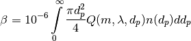
$\beta=10^{-6} \int\limits_{0}^{\infty}\frac{\pi d_p^2}{4}Q(m,\lambda,d_p)n(d_p)dd_p$

where d_p is the diameter of the particle (in nm), n(d_p) is the number of particles of diameter d_p (per cubic centimeter), and the factor 10^-6 is used to cast the result in units of Mm^-1.

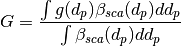
The bulk asymmetry parameter G is calculated by:

$G=\frac{\int g(d_p)\beta_{sca}(d_p)dd_p}{\int \beta_{sca}(d_p)dd_p}$

There is an important distinction in how the size distribution is reported from an instrument vs. the way it is computed analytically. From a laboratory instruments such as an SMPS, total N is the sum of the concentrations in each bin. When computed analytically, total N is the integral area. This can cause issues when dealing with laboratory data, and so a new parameter SMPS is introduced as of version 1.8.0. SMPS is assumed True, that is, PyMieScatt assumes laboratory measurements by default. Set this parameter to False when dealing with theoretical data from analytical distribution functions.

Mie_SD(m, wavelength, sizeDistributionDiameterBins, sizeDistribution[, nMedium=1.0, SMPS=True, asDict=False])¶

Returns Mie coefficients β_ext, β_sca, β_abs, G, β_pr, β_back, β_ratio. Uses scipy.integrate.trapz to compute the integral, which can introduce errors if your distribution is too sparse. Best used with a continuous, compactly-supported distribution.

Parameters

m : complex: The complex refractive index, with the convention m = n+ik.
wavelength : float: The wavelength of incident light, in nanometers.
sizeDistributionDiameterBins : list, tuple, or numpy.ndarray: The diameter bin midpoints of the size distribution, in nanometers.
sizeDistribution : list, tuple, or numpy.ndarray: The number concentrations of the size distribution bins. Must be the same size as sizeDistributionDiameterBins.
nMedium : float, optional: The refractive index of the surrounding medium. This must be positive, nonzero, and real. Any imaginary part will be discarded.
SMPS : bool, optional: The switch determining the source of the size distribution data. Omit or set to True for laboratory measurements, set to False for analytical distributions.
asDict : bool, optional: If specified and set to True, returns the results as a dict.

Returns

Bext, Bsca, Babs, G, Bpr, Bback, Bratio : float: The Mie coefficients calculated by AutoMieQ(), integrated over the size distribution.
q : dict: If asDict==True, MieQ_SD() returns a dict of the above values with appropriate keys.

Mie_Lognormal(m, wavelength, geoStdDev, geoMean, numberOfParticles[, nMedium=1.0, numberOfBins=1000, lower=1, upper=1000, gamma=[1], returnDistribution=False, decomposeMultimodal=False, asDict=False])¶

Returns Mie coefficients $\beta_{ext}$ , $\beta_{sca}$ , $\beta_{abs}$ , $G$ , $\beta_{pr}$ , $\beta_{back}$ , and $\beta_{ratio}$ , integrated over a mathematically-generated k-modal lognormal particle number distribution. Uses scipy.integrate.trapz to compute the integral.

The general form of a k-modal lognormal distribution is given by:

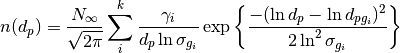
$n(d_p)=\frac{N_\infty}{\sqrt{2\pi}} \sum_{i}^{k}\frac{\gamma_i}{d_p\ln\sigma_{g_i}}\exp\left\{ \frac{-(\ln d_p-\ln d_{pg_i})^2}{2 \ln^2\sigma_{g_i}}\right\}$

where $d_{p}$ is the diameter of the particle (in nm), $n(d_{p})$ is the number of particles of diameter $d_{p}$ (per cubic centimeter), $N_\infty$ is the total number of particles in the distribution, $\sigma_{g_i}$ is the geometric standard deviation of mode $i$ , and $d_{pg_i}$ is the geometric mean diameter (in nm) of the i^th moment. $\gamma_i$ is a porportionality constant that determines the fraction of total particles in the i^th moment.

This function is essentially a wrapper for Mie_SD(). A warning will be raised if the distribution is not compactly-supported on the interval specified by lower and upper.

Parameters

m : complex: The complex refractive index, with the convention m = n+ik.
wavelength : float: The wavelength of incident light, in nanometers.
geoStdDev : float or list-like: The geometric standard deviation(s) $\sigma_g$ or $\sigma_{g_i}$ if list-like.
geoMean : float or list-like: The geometric mean diameter(s) $d_{pg}$ or $d_{pg_i}$ if list-like, in nanometers.
numberOfParticles : float: The total number of particles in the distribution.
nMedium : float, optional: The refractive index of the surrounding medium. This must be positive, nonzero, and real. Any imaginary part will be discarded.
numberOfBins : int, optional: The number of discrete bins in the distribution. Defaults to 1000.
lower : float, optional: The smallest diameter bin, in nanometers. Defaults to 1 nm.
upper : float, optional: The largest diameter bin, in nanometers. Defaults to 1000 nm.
gamma : list-like, optional: The porportionality coefficients for dividing total particles among modes.
returnDistribution : bool, optional: If True, both the size distribution bins and number concentrations will be returned.
decomposeMultimodal: bool, optional: If True (and returnDistribution==True), then the function returns an additional parameter containing the individual modes of the distribution.
asDict : bool, optional: If True, returns the results as a dict.

Returns

Bext, Bsca, Babs, G, Bpr, Bback, Bratio : float: The Mie coefficients calculated by MieQ(), integrated over the size distribution.
diameters, nd : numpy.ndarray: The diameter bins and number concentrations per bin, respectively. Only if returnDistribution is True.
ndi : list of numpy.ndarray objects: A list whose entries are the individual modes that created the multimodal distribution. Only returned if both returnDistribution and decomposeMultimodal are True.
B : dict: If asDict==True, MieQ_withLognormalDistribution() returns a dict of the above values with appropriate keys.

For example, compute the Mie coefficients of a lognormal size distribution with 1000000 particles, σ_g = 1.7, and d_pg = 200 nm; with m = 1.60+0.08i and λ = 532 nm:

>>> import PyMieScatt as ps
>>> ps.MieQ_Lognormal(1.60+0.08j,532,1.7,200,1e6,asDict=True)
{'Babs': 33537.324569179938,
'Bback': 10188.473118449627,
'Bext': 123051.1109783932,
'Bpr': 62038.347528346232,
'Bratio': 12701.828124508347,
'Bsca': 89513.786409213266,
'bigG': 0.6816018615403715}

Angular Functions¶

These functions compute the angle-dependent scattered field intensities and scattering matrix elements. They return arrays that are useful for plotting.

ScatteringFunction(m, wavelength, diameter[, nMedium=1.0, minAngle=0, maxAngle=180, angularResolution=0.5, space='theta', angleMeasure='radians', normalization=None])¶

Creates arrays for plotting the angular scattering intensity functions in theta-space with parallel, perpendicular, and unpolarized light. Also includes an array of the angles for each step. This angle can be in either degrees, radians, or gradians for some reason. The angles can either be geometrical angle or the qR vector (see Sorensen, M. Q-space analysis of scattering by particles: a review. J. Quant. Spectrosc. Radiat. Transfer 2013, 131, 3-12). Uses MieS1S2() to compute S₁ and S₂, then computes parallel, perpendicular, and unpolarized intensities by

$SL(\theta)=|S_1|^2$

$SR(\theta)=|S_2|^2$

$SU(\theta)=\frac{1}{2}(SR+SL)$

Parameters

m : complex

The complex refractive index with the convention m = n+ik.

wavelength : float

The wavelength of incident light, in nanometers.

diameter : float

The diameter of the particle, in nanometers.

nMedium : float, optional

The refractive index of the surrounding medium. This must be positive, nonzero, and real. Any imaginary part will be discarded.

minAngle : float, optional

The minimum scattering angle (in degrees) to be calculated. Defaults to 0.

maxAngle : float, optional

The maximum scattering angle (in degrees) to be calculated. Defaults to 180.

angularResolution : float, optional

The resolution of the output. Defaults to 0.5, meaning a value will be calculated for every 0.5 degrees.

space : str, optional

The measure of scattering angle. Can be ‘theta’ or ‘qspace’. Defaults to ‘theta’.

angleMeasure : str, optional

The units for the scattering angle

normalization : str or None, optional

Specifies the normalization method, which is either by total signal or maximum signal.

normalization = ‘t’ will normalize by the total integrated signal, that is, the total signal will have an integrated value of 1.
normalization = ‘max’ will normalize by the maximum value of the signal regardless of the angle at which it occurs, that is, the maximum signal at that angle will have a value of 1.

Returns

theta : numpy.ndarray: An array of the angles used in calculations. Values will be spaced according to angularResolution, and the size of the array will be (maxAngle-minAngle)/angularResolution.
SL : numpy.ndarray: An array of the scattered intensity of left-polarized (perpendicular) light. Same size as the theta array.
SR : numpy.ndarray: An array of the scattered intensity of right-polarized (parallel) light. Same size as the theta array.
SU : numpy.ndarray: An array of the scattered intensity of unpolarized light, which is the average of SL and SR. Same size as the theta array.

SF_SD(m, wavelength, dp, ndp[, nMedium=1.0, minAngle=0, maxAngle=180, angularResolution=0.5, space='theta', angleMeasure='radians', normalization=None])¶

Creates arrays for plotting the angular scattering intensity functions in theta-space with parallel, perpendicular, and unpolarized light. Also includes an array of the angles for each step for a distribution n_d(d_p). Uses ScatteringFunction() to compute scattering for each particle size, then sums the contributions from each bin.

Parameters

m : complex

The complex refractive index with the convention m = n+ik.

wavelength : float

The wavelength of incident light, in nanometers.

dp : list-like

The diameter bins of the distribution, in nanometers.

ndp : list-like

The number of particles in each diameter bin in dp.

nMedium : float, optional

The refractive index of the surrounding medium. This must be positive, nonzero, and real. Any imaginary part will be discarded.

minAngle : float, optional

The minimum scattering angle (in degrees) to be calculated. Defaults to 0.

maxAngle : float, optional

The maximum scattering angle (in degrees) to be calculated. Defaults to 180.

angularResolution : float, optional

The resolution of the output. Defaults to 0.5, meaning a value will be calculated for every 0.5 degrees.

space : str, optional

The measure of scattering angle. Can be ‘theta’ or ‘qspace’. Defaults to ‘theta’.

angleMeasure : str, optional

The units for the scattering angle

normalization : str or None, optional

Specifies the normalization method, which is either by total particle number, total signal or maximum signal.

normalization = ‘n’ will normalize by the total number of particles (the integral of the size distribution). Can lead to weird interpretations, so use caution.
normalization = ‘t’ will normalize by the total integrated signal, that is, the total signal will have an integrated value of 1.
normalization = ‘max’ will normalize by the maximum value of the signal regardless of the angle at which it occurs, that is, the maximum signal at that angle will have a value of 1.

Returns

theta : numpy.ndarray: An array of the angles used in calculations. Values will be spaced according to angularResolution, and the size of the array will be (maxAngle-minAngle)/angularResolution.
SL : numpy.ndarray: An array of the scattered intensity of left-polarized (perpendicular) light. Same size as the theta array.
SR : numpy.ndarray: An array of the scattered intensity of right-polarized (parallel) light. Same size as the theta array.
SU : numpy.ndarray: An array of the scattered intensity of unpolarized light, which is the average of SL and SR. Same size as the theta array.

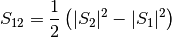
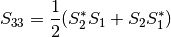
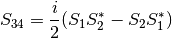
MatrixElements(m, wavelength, diameter, mu[, nMedium=1.0])¶

Calculates the four nonzero scattering matrix elements S₁₁, S₁₂, S₃₃, and S₃₄ as functions of μ=cos(θ), where θ is the scattering angle:

$S_{11}=\frac{1}{2}\left(|S_2|^2+|S_1|^2\right)$

$S_{12}=\frac{1}{2}\left(|S_2|^2-|S_1|^2\right)$

$S_{33}=\frac{1}{2}(S_2^*S_1+S_2S_1^*)$

$S_{34}=\frac{i}{2}(S_1S_2^*-S_2S_1^*)$

Parameters

m : complex: The complex refractive index with the convention m = n+ik.
wavelength : float: The wavelength of incident light, in nanometers.
diameter : float: The diameter of the particle, in nanometers.
mu : float: The cosine of the scattering angle.
nMedium : float, optional: The refractive index of the surrounding medium. This must be positive, nonzero, and real. Any imaginary part will be discarded.

Returns

S11, S12, S33, S34 : float: The matrix elements described above.

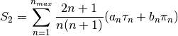
MieS1S2(m, x, mu)¶

Calculates S₁ and S₂ at μ=cos(θ), where θ is the scattering angle.

Uses Mie_ab() to calculate a_n and b_n, and MiePiTau() to calculate π_n and τ_n. S₁ and S₂ are calculated by: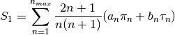

$S_1=\sum\limits_{n=1}^{n_{max}}\frac{2n+1}{n(n+1)}(a_n\pi_n+b_n\tau_n)$

$S_2=\sum\limits_{n=1}^{n_{max}}\frac{2n+1}{n(n+1)}(a_n\tau_n+b_n\pi_n)$

Parameters

m : complex: The complex refractive index with the convention m = n+ik.
x : float: The size parameter $x=\pi\,d_p/\lambda$ .
mu : float: The cosine of the scattering angle.

Returns

S1, S2 : complex: The S₁ and S₂ values.

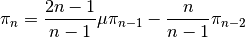
MiePiTau(mu, nmax)¶

Calculates π_n and τ_n.

This function uses recurrence relations to calculate π_n and τ_n, beginning with π₀ = 1, π₁ = 3μ (where μ is the cosine of the scattering angle), τ₀ = μ, and τ₁ = 3cos(2cos^-1 (μ)):

$\pi_n=\frac{2n-1}{n-1}\mu\pi_{n-1}-\frac{n}{n-1}\pi_{n-2}$

$\tau_n=n\mu\pi_n-(n+1)\pi_{n-1}$

Parameters

mu : float: The cosine of the scattering angle.
nmax : int: The number of elements to compute. Typically, n_max = floor(2+x+4x^1/3), but can be given any integer.

Returns

p, t : numpy.ndarray: The π_n and τ_n arrays, of length nmax.