General Usage tips and Example Scripts

Examples are now more or less up-to-date with PyMieScatt’s modern syntax.

PyMieScatt’s functions are designed to work as a standalone calculator or as part of larger, more customized scripts. This page has a few selected examples which will expand as more innovative use cases appear. If you use PyMieScatt in your research in an unexpected or novel way, please contact the author to post an example here.

Mie Efficiencies of a Single Homogeneous Particle

To calculate the efficencies of a single homogeneous particle, use the MieQ() function.

>>> import PyMieScatt as ps
>>> ps.MieQ(1.5+0.5j,532,200,asDict=True)
{'Qabs': 1.2206932456722366,
 'Qback': 0.2557593071989655,
 'Qext': 1.6932375984850729,
 'Qpr': 1.5442174328606282,
 'Qratio': 0.5412387338385265,
 'Qsca': 0.47254435281283641,
 'g': 0.3153569918620277}

Mie Efficencies of a Weibull Distribution

Consider the 405 nm Mie coefficients of 105 particles/cm³, with m = 1.5+0.5i, in a Weibull distribution with shape parameter sh = 5 and scale parameter sc = 200:

>>> import PyMieScatt as ps
>>> import numpy as np
>>> import matplotlib.pyplot as plt
>>> dp = np.linspace(10,1000,1000)
>>> N,sh,sc = 1e5,5,200
>>> w=[N*((sh/sc)*(d/sc)**(sh-1))*np.exp(-(d/sc)**sh) for d in dp]
>>> ps.Mie_SD(1.5+0.5j,405,dp,w,asDict=True,SMPS=False)
{'Babs': 3762.0479602613427,
 'Bback': 286.65698999981691,
 'Bext': 5747.4466502095638,
 'Bpr': 4662.181554274106,
 'Bratio': 550.87163111634698,
 'Bsca': 1985.3986899482211,
 'G': 0.54662325578736115}

Plotting Angular Functions

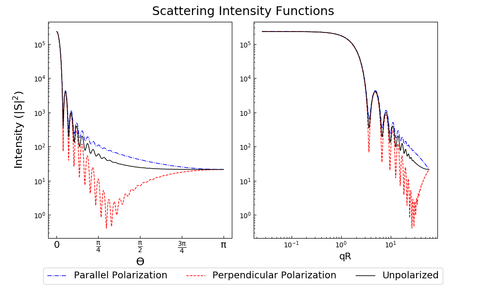
The angular functions return arrays that are suitable for plotting with MatPlotLib. For example, plot the angular scattering functions of a 5 μm particle with m=1.7+0.5i, illuminated by 532 nm light. Note that the Mie calculations themselves only need two lines, the rest is making the plot look nice:

import PyMieScatt as ps
import numpy as np
import matplotlib.pyplot as plt

m=1.7+0.5j
w=532
d=5000

theta,SL,SR,SU = ps.ScatteringFunction(m,w,d)
qR,SLQ,SRQ,SUQ = ps.ScatteringFunction(m,w,d,space='qspace')

plt.close('all')

fig1 = plt.figure(figsize=(10,6))
ax1 = fig1.add_subplot(1,2,1)
ax2 = fig1.add_subplot(1,2,2)

ax1.semilogy(theta,SL,'b',ls='dashdot',lw=1,label="Parallel Polarization")
ax1.semilogy(theta,SR,'r',ls='dashed',lw=1,label="Perpendicular Polarization")
ax1.semilogy(theta,SU,'k',lw=1,label="Unpolarized")

x_label = ["0", r"$\mathregular{\frac{\pi}{4}}$", r"$\mathregular{\frac{\pi}{2}}$",r"$\mathregular{\frac{3\pi}{4}}$",r"$\mathregular{\pi}$"]
x_tick = [0,np.pi/4,np.pi/2,3*np.pi/4,np.pi]
ax1.set_xticks(x_tick)
ax1.set_xticklabels(x_label,fontsize=14)
ax1.tick_params(which='both',direction='in')
ax1.set_xlabel("ϴ",fontsize=16)
ax1.set_ylabel(r"Intensity ($\mathregular{|S|^2}$)",fontsize=16,labelpad=10)

ax2.loglog(qR,SLQ,'b',ls='dashdot',lw=1,label="Parallel Polarization")
ax2.loglog(qR,SRQ,'r',ls='dashed',lw=1,label="Perpendicular Polarization")
ax2.loglog(qR,SUQ,'k',lw=1,label="Unpolarized")

ax2.tick_params(which='both',direction='in')
ax2.set_xlabel("qR",fontsize=14)
handles, labels = ax1.get_legend_handles_labels()
fig1.legend(handles,labels,fontsize=14,ncol=3,loc=8)

fig1.suptitle("Scattering Intensity Functions",fontsize=18)
fig1.show()
plt.tight_layout(rect=[0.01,0.05,0.915,0.95])

This produces the following image:

We can do better, though! Suppose we wanted to, for educational purposes, demonstrate how the “Mie ripples” develop as we increase size parameter. This script considers a weakly absorbing particle of m=1.536+0.0015i. Its size parameter increases from 0.08 to 500 nm, the scattering function is plotted and a figure file is saved. The final few lines gather the figures into an mp4 video. Note that the Mie mathematics need only one line per loop, and the rest is generating images and movies.

First, install ffmpeg exe using conda: .. code-block:

$ conda install ffmpeg -c conda-forge

import PyMieScatt as ps
import numpy as np
import matplotlib.pyplot as plt
import imageio
import os

wavelength=450.0
m=1.536+0.0015j
drange = np.logspace(1,np.log10(500*405/np.pi),250)
for i,d in enumerate(drange):
  if 250%(i+1)==0:
    print("Working on image " + str(i) + "...",flush=True)
  theta,SL,SR,SU = ps.ScatteringFunction(m,wavelength,d,space='theta',normalization='t')

  plt.close('all')

  fig1 = plt.figure(figsize=(10.08,6.08))
  ax1 = fig1.add_subplot(1,1,1)
  #ax2 = fig1.add_subplot(1,2,2)

  ax1.semilogy(theta,SL,'b',ls='dashdot',lw=1,label="Parallel Polarization")
  ax1.semilogy(theta,SR,'r',ls='dashed',lw=1,label="Perpendicular Polarization")
  ax1.semilogy(theta,SU,'k',lw=1,label="Unpolarized")

  x_label = ["0", r"$\mathregular{\frac{\pi}{4}}$", r"$\mathregular{\frac{\pi}{2}}$",r"$\mathregular{\frac{3\pi}{4}}$",r"$\mathregular{\pi}$"]
  x_tick = [0,np.pi/4,np.pi/2,3*np.pi/4,np.pi]
  ax1.set_xticks(x_tick)
  ax1.set_xticklabels(x_label,fontsize=14)
  ax1.tick_params(which='both',direction='in')
  ax1.set_xlabel("ϴ",fontsize=16)
  ax1.set_ylabel(r"Intensity ($\mathregular{|S|^2}$)",fontsize=16,labelpad=10)
  ax1.set_ylim([1e-9,1])
  ax1.set_xlim([1e-3,theta[-1]])
  ax1.annotate("x = πd/λ = {dd:1.2f}".format(dd=np.round(np.pi*d/405,2)), xy=(3, 1e-6),  xycoords='data',
            xytext=(0.05, 0.1), textcoords='axes fraction',
            horizontalalignment='left', verticalalignment='top',
            fontsize=18
            )
  handles, labels = ax1.get_legend_handles_labels()
  fig1.legend(handles,labels,fontsize=14,ncol=3,loc=8)

  fig1.suptitle("Scattering Intensity Functions",fontsize=18)
  fig1.show()
  plt.tight_layout(rect=[0.01,0.05,0.915,0.95])

  plt.savefig('output\\' + str(i).rjust(3,'0') + '.png')

filenames = os.listdir('output\\')
dur = [0.1 for x in range(250)]
dur[249]=10
with imageio.get_writer('mie_ripples.mp4', mode='I', fps=10) as writer:
    for filename in filenames:
        image = imageio.imread('output\\' + filename)
        writer.append_data(image)

This produces a nice video, which I’ll embed here just as soon as ReadTheDocs supports Github content embedding. For now, you can download it here.

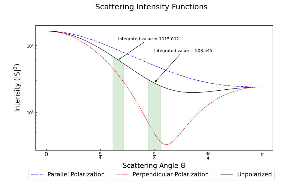
Angular Scattering Function of Salt Aerosol

Recently, a colleague needed to know how much light a distribution of salt aerosol would scatter into two detectors, one at 60° and one at 90°. We modeled a lognormal distribution of NaCl particles based on laboratory measurements and then tried to figure out how much light we’d see at various angles.

import PyMieScatt as ps # import PyMieScatt and abbreviate as ps
import matplotlib.pyplot as plt # import standard plotting library and abbreviate as plt
import numpy as np # import numpy and abbreviate as np
from scipy.integrate import trapz # import a single function for integration using trapezoidal rule

m = 1.536 # refractive index of NaCl
wavelength = 405 # replace with the laser wavelength (nm)

dp_g = 85 # geometric mean diameter - replace with your own (nm)
sigma_g = 1.5 # geometric standard deviation - replace with your own (unitless)
N = 1e5 # total number of particles - replace with your own (cm^-3)

B = ps.Mie_Lognormal(m,wavelength,sigma_g,dp_g,N,numberOfBins=1000,returnDistribution=True) # Calculate optical properties

S = ps.SF_SD(m,wavelength,B[7],B[8])

#%% Make graphs - lots of this is really unnecessary decoration for a pretty graph.
plt.close('all')

fig1 = plt.figure(figsize=(10.08,6.08))
ax1 = fig1.add_subplot(1,1,1)

ax1.plot(S[0],S[1],'b',ls='dashdot',lw=1,label="Parallel Polarization")
ax1.plot(S[0],S[2],'r',ls='dashed',lw=1,label="Perpendicular Polarization")
ax1.plot(S[0],S[3],'k',lw=1,label="Unpolarized")

x_label = ["0", r"$\mathregular{\frac{\pi}{4}}$", r"$\mathregular{\frac{\pi}{2}}$",r"$\mathregular{\frac{3\pi}{4}}$",r"$\mathregular{\pi}$"]
x_tick = [0,np.pi/4,np.pi/2,3*np.pi/4,np.pi]
ax1.set_xticks(x_tick)
ax1.set_xticklabels(x_label,fontsize=14)
ax1.tick_params(which='both',direction='in')
ax1.set_xlabel("Scattering Angle ϴ",fontsize=16)
ax1.set_ylabel(r"Intensity ($\mathregular{|S|^2}$)",fontsize=16,labelpad=10)
handles, labels = ax1.get_legend_handles_labels()
fig1.legend(handles,labels,fontsize=14,ncol=3,loc=8)

fig1.suptitle("Scattering Intensity Functions",fontsize=18)
fig1.show()
plt.tight_layout(rect=[0.01,0.05,0.915,0.95])

# Highlight certain angles and compute integral
sixty = [0.96<x<1.13 for x in S[0]]
ninety = [1.48<x<1.67 for x in S[0]]
ax1.fill_between(S[0],0,S[3],where=sixty,color='g',alpha=0.15)
ax1.fill_between(S[0],0,S[3],where=ninety,color='g',alpha=0.15)
ax1.set_yscale('log')

int_sixty = trapz(S[3][110:130],S[0][110:130])
int_ninety = trapz(S[3][169:191],S[0][169:191])

# Annotate plot with integral results
ax1.annotate("Integrated value = {i:1.3f}".format(i=int_sixty),
            xy=(np.pi/3, S[3][120]), xycoords='data',
            xytext=(np.pi/3, 12000), textcoords='data',
            arrowprops=dict(arrowstyle="->",
                            connectionstyle="arc3"),
            )
ax1.annotate("Integrated value = {i:1.3f}".format(i=int_ninety),
            xy=(np.pi/2, S[3][180]), xycoords='data',
            xytext=(np.pi/2, 8000), textcoords='data',
            arrowprops=dict(arrowstyle="->",
                            connectionstyle="arc3"),
            )

Modeling Behavior of a Self-Preserving Distribution

This code example will (after several hours on a typical PC) produce a ten-second video of the scattering and absorption behavior of a δ-distribution of 300 nm particles, which can be considered the limiting case of a lognormal distribution where the geometric standard deviation σ_g equals 1. Atmospheric aerosol distributions are typically modeled as lognormal distributions with σ_g around 1.7, and here we animate from 1 to 2. The animation also includes the solution for the refractive index given some assumed optical measurements (that is, scattering and absorption measurements when m=1.60+0.36j and λ = 405 nm).

There is a commented block on lines 37-39 that can be uncommented to produce a single image with random σ_g between 1 and 2. The revelent PyMieScatt calculations are on lines 45 and 136. That’s it! The rest is preparing inputs and making pretty graphs.

I’m still working on optimizing a few things. For now, it takes about 15 minutes to make each frame on my computer. At 50 frames, that’s about 12.5 hours.

import PyMieScatt as ps
import matplotlib.pyplot as plt
import numpy as np
from time import time
import matplotlib.colors as colors
from mpl_toolkits.mplot3d import Axes3D
from matplotlib import cm
from scipy.ndimage import zoom
import imageio
import os

def truncate_colormap(cmap, minval=0.0, maxval=1.0, n=100):
  new_cmap = colors.LinearSegmentedColormap.from_list('trunc({n},{a:.2f},{b:.2f})'.format(n=cmap.name, a=minval, b=maxval),cmap(np.linspace(minval, maxval, n)))
  return new_cmap

N = 1e6
w = 405
maxDiameter = 3500
numDiams = 1200

ithPart = lambda gammai, dp, dpgi, sigmagi: (gammai/(np.sqrt(2*np.pi)*np.log(sigmagi)*dp))*np.exp(-(np.log(dp)-np.log(dpgi))**2/(2*np.log(sigmagi)**2))
dp = np.logspace(np.log10(1), np.log10(maxDiameter), numDiams)

sigmaList = np.logspace(np.log10(1.005), np.log10(2), 49)

mu=300

ndp = [N*ithPart(1,dp,mu,s) for s in sigmaList]

deltaD = np.zeros(numDiams)
deltaD[838]=N

lognormalList = [deltaD] + ndp
sigmaList = np.insert(sigmaList,0,1)

## Test region - uncomment for a single graph
#testCase = np.random.randint(1,49)
#lognormalList = [lognormalList[testCase]]
#sigmaList = [sigmaList[testCase]]

BscaSolution = []
BabsSolution = []

for l in lognormalList:
  _,_s,_a,*rest = ps.Mie_SD(1.6+0.36j,w,dp,l)
  BscaSolution.append(_s)
  BabsSolution.append(_a)

nMin=1.3
nMax=3
kMin=0
kMax=2

points = 40
interpolationFactor = 2

nRange = np.linspace(nMin,nMax,points)
kRange = np.linspace(kMin,kMax,points)

plt.close('all')

for i,(sigma,l,ssol,asol) in enumerate(zip(sigmaList,lognormalList,BscaSolution,BabsSolution)):
  start = time()
  BscaList = []
  BabsList = []
  nList = []
  kList = []
  for n in nRange:
    s = []
    a = []
    for k in kRange:
      m = n+k*1.0j
      _,Bsca,Babs,*rest = ps.Mie_SD(m,w,dp,l)
      s.append(Bsca)
      a.append(Babs)
    BscaList.append(s)
    BabsList.append(a)
  n = zoom(nRange,interpolationFactor)
  k = zoom(kRange,interpolationFactor)
  BscaSurf = zoom(np.transpose(np.array(BscaList)),interpolationFactor)
  BabsSurf = zoom(np.transpose(np.array(BabsList)),interpolationFactor)
  nSurf,kSurf=np.meshgrid(n,k)

  c1 = truncate_colormap(cm.Reds,0.2,1,n=256)
  c2 = truncate_colormap(cm.Blues,0.2,1,n=256)

  xMin,xMax = nMin,nMax
  yMin,yMax = kMin,kMax

  plt.close('all')
  fig1 = plt.figure(figsize=(10.08,8))

  plt.suptitle("σ={ww:1.3f}".format(ww=sigma),fontsize=24)

  ax1 = plt.subplot2grid((3,4),(0,0), projection='3d', rowspan=2, colspan=2)
  ax2 = plt.subplot2grid((3,4),(0,2), projection='3d', rowspan=2, colspan=2)
  ax3 = plt.subplot2grid((3,4),(2,0), colspan=3)
  ax4 = plt.subplot2grid((3,4),(2,3))

  ax1.plot_surface(nSurf,kSurf,BscaSurf,rstride=1,cstride=1,cmap=c1,alpha=0.5)
  ax1.contour(nSurf,kSurf,BscaSurf,[ssol],lw=2,colors='r',linestyles='dashdot')
  ax1.contour(nSurf,kSurf,BscaSurf,[ssol],colors='r',linestyles='dashdot',offset=0)

  ax2.plot_surface(nSurf,kSurf,BabsSurf,rstride=1,cstride=1,cmap=c2,alpha=0.5,zorder=-1)
  ax2.contour(nSurf,kSurf,BabsSurf,[asol],lw=2,colors='b',linestyles='solid',zorder=3)
  ax2.contour(nSurf,kSurf,BabsSurf,[asol],colors='b',linestyles='solid',offset=0)

  boxLabels = ["βsca","βabs"]

  yticks = [2,1.5,1,0.5,0]
  xticks = [3,2.5,2,1.5]

  for a,t in zip([ax1,ax2],boxLabels):
    lims = a.get_zlim3d()
    a.set_zlim3d(0,lims[1])
    a.text(1.5,0,(a.get_zlim3d()[1])*1.15,t,ha="center",va="center",size=18,zorder=5)
    a.set_ylim(2,0)
    a.set_xlim(3,1.3)
    a.set_xticks(xticks)
    a.set_xticklabels(xticks,rotation=-15,va='center',ha='left')
    a.set_yticks(yticks)
    a.set_yticklabels(yticks,rotation=-15,va='center',ha='left')
    a.set_zticklabels([])
    a.view_init(20,120)
    a.tick_params(axis='both', which='major', labelsize=12,pad=0)
    a.tick_params(axis='y',pad=-2)
    a.set_xlabel("n",fontsize=18,labelpad=2)
    a.set_ylabel("k",fontsize=18,labelpad=3)

  ax3.semilogx(dp,l,c='g')
  ax3.set_xlabel('Diameter',fontsize=16)
  ax3.get_yaxis().set_ticks([])
  ax3.tick_params(which='both',direction='in')
  ax3.grid(color='#dddddd')

  giv = ps.ContourIntersection_SD(ssol,asol,w,dp,l,gridPoints=points*1.5,kMin=0.001,kMax=2,axisOption=10,fig=fig1,ax=ax4)
  ax4.set_xlim(1.3,3)
  ax4.yaxis.tick_right()
  ax4.yaxis.set_label_position("right")
  ax4.legend_.remove()
  ax4.set_title("")
  ax4.set_yscale('linear')

  plt.tight_layout()

  plt.savefig("Distro/{num:02d}_distro.png".format(num=i))

  end = time()
  print("Frame {n:1d}/30 done in {t:1.2f} seconds.".format(n=i+1,t=end-start))

filenames = os.listdir('Distro\\')
with imageio.get_writer('SD.mp4', mode='I', fps=5) as writer:
  for filename in filenames:
    image = imageio.imread('Distro\\' + filename)
    writer.append_data(image)

Once readthedocs allows embedded .mp4s, the animation will be posted here. I should probably just make a youtube account.

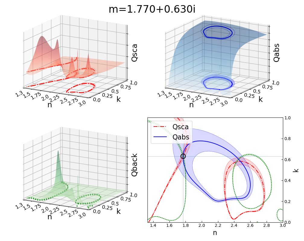
Visualization of the Contour Intersection Inversion Method

This example illustrates the algorithm used by the contour intersection method. It will plot the Qabs, Qsca, and Qback surface and show how the measurement contours intersect in n-k space. The inversion algorithm only generates the lower-right plot on line 126 of this script. The rest is entirely illustrative, but uses forward Mie calculations in the loop on line 46. This script requires significant overhead from matplotlib (even more so since the 2.1 update). The actual inversion algorithm runs much faster.

import PyMieScatt as ps
import matplotlib.pyplot as plt
import numpy as np
from time import time
import matplotlib.colors as colors
from mpl_toolkits.mplot3d import Axes3D
from matplotlib import cm
from scipy.ndimage import zoom

def truncate_colormap(cmap, minval=0.0, maxval=1.0, n=100):
  new_cmap = colors.LinearSegmentedColormap.from_list('trunc({n},{a:.2f},{b:.2f})'.format(n=cmap.name, a=minval, b=maxval),cmap(np.linspace(minval, maxval, n)))
  return new_cmap

d = 300
w = 375
m = 1.77+0.63j

nMin=1.33
nMax=3
kMin=0.001
kMax=1
err = 0.01

Qm = ps.fastMieQ(m,w,d)

points = 200
interpolationFactor = 2

nRange = np.linspace(nMin,nMax,points)
kRange = np.linspace(kMin,kMax,points)

plt.close('all')

start = time()
QscaList = []
QabsList = []
QbackList = []
nList = []
kList = []
for n in nRange:
  s = []
  a = []
  b = []
  for k in kRange:
    m = n+k*1.0j
    Qsca,Qabs,Qback = ps.fastMieQ(m,w,d)
    s.append(Qsca)
    a.append(Qabs)
    b.append(Qback)
  QscaList.append(s)
  QabsList.append(a)
  QbackList.append(b)
n = zoom(nRange,interpolationFactor)
k = zoom(kRange,interpolationFactor)
QscaSurf = zoom(np.transpose(np.array(QscaList)),interpolationFactor)
QabsSurf = zoom(np.transpose(np.array(QabsList)),interpolationFactor)
QbackSurf = zoom(np.transpose(np.array(QbackList)),interpolationFactor)

nSurf,kSurf=np.meshgrid(n,k)

c1 = truncate_colormap(cm.Reds,0.2,1,n=256)
c2 = truncate_colormap(cm.Blues,0.2,1,n=256)
c3 = truncate_colormap(cm.Greens,0.2,1,n=256)

xMin,xMax = nMin,nMax
yMin,yMax = kMin,kMax

plt.close('all')
fig1 = plt.figure(figsize=(10.08,8))

ax1 = plt.subplot2grid((2,2),(0,0), projection='3d')
ax2 = plt.subplot2grid((2,2),(0,1), projection='3d')
ax3 = plt.subplot2grid((2,2),(1,0), projection='3d')
ax4 = plt.subplot2grid((2,2),(1,1))
ax1.set_proj_type('ortho')
ax2.set_proj_type('ortho')
ax3.set_proj_type('ortho')

qscaerrs = [Qm[0]-Qm[0]*err,Qm[0]+Qm[0]*err]
qabserrs = [Qm[1]-Qm[1]*err,Qm[1]+Qm[1]*err]
qbackerrs = [Qm[2]-Qm[2]*err,Qm[2]+Qm[2]*err]

ax1.plot_surface(nSurf,kSurf,QscaSurf,rstride=1,cstride=1,cmap=c1,alpha=0.5)
ax1.contour(nSurf,kSurf,QscaSurf,Qm[0],linewidths=2,colors='r',linestyles='dashdot')
ax1.contour(nSurf,kSurf,QscaSurf,qscaerrs,linewidths=0.5,colors='r',linestyles='dashdot',alpha=0.75)
ax1.contour(nSurf,kSurf,QscaSurf,Qm[0],linewidths=2,colors='r',linestyles='dashdot',offset=0)
ax1.contourf(nSurf,kSurf,QscaSurf,qscaerrs,colors='r',offset=0,alpha=0.25)

ax2.plot_surface(nSurf,kSurf,QabsSurf,rstride=1,cstride=1,cmap=c2,alpha=0.5)
ax2.contour(nSurf,kSurf,QabsSurf,Qm[1],linewidths=2,colors='b',linestyles='solid')
ax2.contour(nSurf,kSurf,QabsSurf,qabserrs,linewidths=0.5,colors='b',linestyles='solid',alpha=0.75)
ax2.contour(nSurf,kSurf,QabsSurf,Qm[1],linewidths=2,colors='b',linestyles='solid',offset=0)
ax2.contourf(nSurf,kSurf,QabsSurf,qabserrs,colors='b',offset=0,alpha=0.25)

ax3.plot_surface(nSurf,kSurf,QbackSurf,rstride=1,cstride=1,cmap=c3,alpha=0.5)
ax3.contour(nSurf,kSurf,QbackSurf,Qm[2],linewidths=2,colors='g',linestyles='dotted')
ax3.contour(nSurf,kSurf,QbackSurf,qbackerrs,linewidths=0.5,colors='g',linestyles='dotted',alpha=0.75)
ax3.contour(nSurf,kSurf,QbackSurf,Qm[2],linewidths=2,colors='g',linestyles='dotted',offset=0)
ax3.contourf(nSurf,kSurf,QbackSurf,qbackerrs,colors='g',offset=0,alpha=0.25)

boxLabels = ["Qsca","Qabs","Qback"]

yticks = np.arange(kMax,kMin-0.25,-0.25)#[1,0.75,0.5,0.25,0]
xticks = np.arange(nMax,1.5-0.25,-0.25)#[2,1.75,1.5,1.25]
xticks = np.append(xticks,1.3)

for a,t in zip([ax1,ax2,ax3],boxLabels):
  lims = a.get_zlim3d()
  a.set_zlim3d(0,lims[1])
  a.set_ylim(kMax,0)
  a.set_yscale('linear')
  a.set_xlim(nMax,1.3)
  a.set_xticks(xticks)
  a.set_xticklabels(xticks,rotation=28,va='bottom',ha='center')
  a.set_yticks(yticks)
  a.set_yticklabels(yticks,rotation=-10,va='center',ha='left')
  a.set_zticklabels([])
  a.view_init(20,120)
  a.tick_params(axis='x', labelsize=12, pad=12)
  a.tick_params(axis='y', labelsize=12, pad=-2)
  a.set_xlabel("n",fontsize=18,labelpad=4)
  a.set_ylabel("k",fontsize=18,labelpad=3)
  a.set_zlabel(t,fontsize=18,labelpad=-10,rotation=90)

Qm = [(q,q*err) for q in Qm]
giv = ps.ContourIntersection(Qm[0],Qm[1],w,d,Qback=Qm[2],gridPoints=200,nMin=nMin,nMax=nMax,kMin=kMin,kMax=kMax,axisOption=1,fig=fig1,ax=ax4)
ax4.set_xlim(nMin,nMax)
ax4.yaxis.tick_right()
ax4.yaxis.set_label_position("right")
ax4.set_title("")
ax4.set_yscale('linear')
l = [giv[-1]['Qsca'],giv[-1]['Qabs'],giv[-1]['Qback']]
[x.set_label(tx) for x,tx in zip(l,boxLabels)]
h = [x.get_label() for x in l]
ax4.legend(l,h,fontsize=16,loc='upper right')

plt.suptitle("m={n:1.3f}+{k:1.3f}i".format(n=giv[0][0].real,k=giv[0][0].imag),fontsize=24)

plt.tight_layout()

#plt.savefig("{n:1.2f}+{k:1.2f}i.png".format(n=giv[0][0].real,k=giv[0][0].imag))

end = time()
print("Done in {t:1.2f} seconds.".format(t=end-start))